Want to read the post in Swedish? Click here

Welcome back, in today’s quite easy post we will take a look at my favourites in the quick access toolbar where we easily can save our favourite commands.

Since we use some commands belonging to the various menu tabs more than others and it is not certain that there is a suitable shortcut, it is a strong recommendation to add these to the toolbar.

The idea with this field is to be able to work quickly and efficiently and I recommend you not to save too many commands here as you risk spending time just looking for the right one. I usually save a maximum of 16 commands depending on what I work with, more than that is not needed since it is good to try to work with shortcuts as much as possible. After learning the shortcut to your favourite, you can delete it.

Look at the lesson in Learnesys course Excel essentials, about the quick access toolbar

This is lesson 3 in Learnesys course Excel essentials, click on the link for more information.

^{Use the voucher code cmkstiller for -15% on all Learnesys’ courses}

Add favourites

Adding your favourites is super-easy, well-invested time and can be done in several ways of which I show three below:

•  Via options
• Via import
•  Via customization
• Via menu tabs

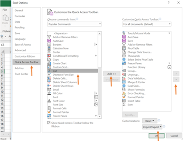
Below you will find the most comprehensive way to add favourites. Via file and options, you find Excel Options where you click the Quick Access Toolbar (arrow 1), then the command you want to add (2) and finally add (3). You can also import a customization file (4) and move up and down (5) the favorites to get them in the order you want.

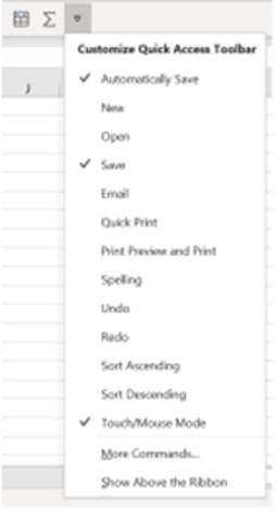
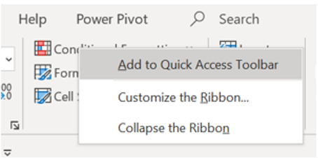
The second fastest way is to click on “Customize the Quick Access Toolbar” in the Quick Access Toolbar as you see in the image above to the right. Click on More Commands. The fastest way you see below where you just right-click on a command under a menu and select add in the Toolbar.

My favourites

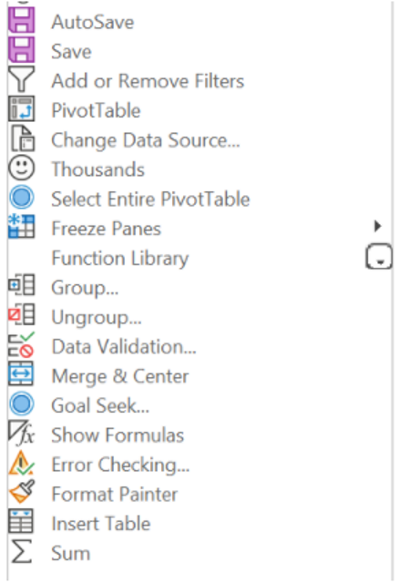
My favourites are the following commands and I recommend you all to find your own favourites and add them.

I have always chosen to show these under the ribbon area to access them as quickly as possible but this is a matter of taste. Automatically, the favourites end up above the menu tabs, but by right-clicking you can check to have them below. You will find explanations for my favourites below. Most are pretty obvious what they do but I will explain what I use some for.

The function library

I have added this library because if you want to and work a lot with formulas, it gives a good overview of the 14 categories of formulas / functions. You can visually see what is in a simple filter list.

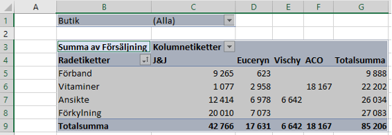
Select the entire PivotTable

This is a very valuable command for me and I often use it when I do reporting. It can be a bit awkward if, for example, you need to delete or move a table to get the right area with you. Then it is time efficient to use this command and I have not been able to find a shortcut for this.

Group and Ungroup

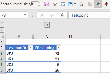
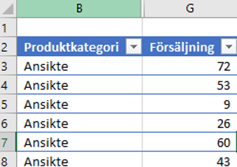
I often use this in large Excel sheets with data as it can be good to be able to group away certain sections temporarily, while it is easy to find these again (see the icon with plus). This without having to look for the area, which you sometimes have to do when you “Hide” a column. See the difference below in the first and second picture. In profit reports with sub-accounts, I usually group the report into groups and sub-groups in order to be able to click out different parts at a detailed level at a time. This is very convenient for results reviews.

• 

• 

Goal Seek

Target search is a function that is very useful in margin analysis or calculations that are made when you have a target number to reach. I used this function continuously in one of my assignments when I worked with profitability analyses at a FMCG company. The function can also be used to an advantage when simulating results in the budget processes.

Show formulas

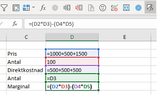
I usually use the function to easily get an overall picture of how a formula is composed together.
This function can be useful if you inherit a file with formulas or take over a calculation that someone has already started or if you need to go back to understand your own logic. I often use the function when I am in a meeting and someone wants to understand more about the steps leading up to the results.

Error checking

I would like to strike a blow for the error checking function. Using this formula, I usually look for any errors that may occur in a sheet with multiple formulas or combinations of formulas. At the same time as you can navigate around and look at the different steps in the formula.

Format Painter

Download format is great as you can quickly select a cell with the brush and pick up the format and then select the area you want to re-format.

Next post

I hope you got some tips from today’s post. In the next post, we will look at how to work with Emojis, which is now part of our way of communicating and which has now entered into Excel.

Feel free to connect with me on LinkedIn and go to Learnesy´s website for more information.

Carl Stiller in collaboration with Learnesy

Use the voucher code cmkstiller for -15% on all Learnesys’ courses!
Go to our shop!