We have now come to the post for the powerful function SUMPRODUCT… my favourite function. I became acquainted with this feature 12 years ago, setting up revenue forecasting models at CA Technologies, and am still finding new ways to use it. This function is said to be one of Excel’s most underrated functions. For an economist/statistician or logistician, this function is invaluable due to its versatility. From the beginning, it was probably not the intention that the function should have such extensive functionality, but it turned out well… for us!

Read the post in Swedish here ??

Look at the lesson in Learnesys course The Excel Functions Guide, about the function SUMPRODUCT

Use the voucher code cmkstiller for -15% on all Learnesys’ courses.
Go to the shop

What is the function used for?

I recommend the SUMPRODUCT to everyone who deals with medium to advanced Excel work as it is a slightly more complicated but extremely useful function. The function can do things that most other functions can do such as OR, NUMBER, VLOOKUP, SUMIFS, INDEX AND MATCH. By exploring what this function can actually do, you will be able to save an incredible amount of time instead of processing data or combining different functions to achieve the same thing.

I use this function for the following work:

• P&L reporting
• Key ratio calculation
• Balanced Scorecard
• Analytical models

How the formula works

The formula is a summation formula where the summation area can have several columns and or several rows. If you compare with SUMIFS, this formula can only look at, for example, a column. You can combine the function with other functions and I will below show 7 ways how I use the formula.

 

Example

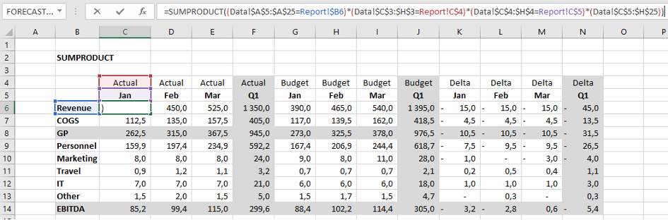
1. Summary with exceptions

I use this method most of all for result reporting or KPI presentations.

The formula is set up to select a row or column in the raw data with factors that you then match against the group accounts or the other factors you have in the report such as scenario and month in our case below. These factors are referred to as “exceptions”.

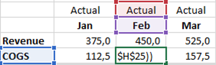
=SUMPRODUCT((Data!$A$5:$A$25=Report!$B6)*(Data!$C$3:$H$3=Report!C$4)*(Data!$C$4:$H$4=Report!C$5)*(Data!$C$5:$H$25))

The first three parts process the factors and the last part “(Data!$C$5:$H$25)” defines the range of amounts below.

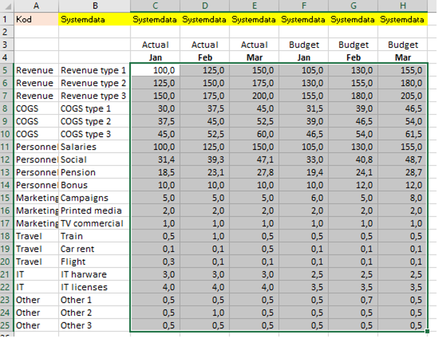
Note that you can also enter the factor that you have in the report with text in the formula;

=SUMPRODUCT((Data!$A$5:$A$25=”Revenue“)*(Data!$C$3:$H$3=Report!C$4)*(Data!$C$4:$H$4=Report!C$5)*(Data!$C$5:$H$25))

This option is often used in SUMIFS formulas. In our case above, we have locked column B, for example, to avoid entering manually the names of the factors for each row.

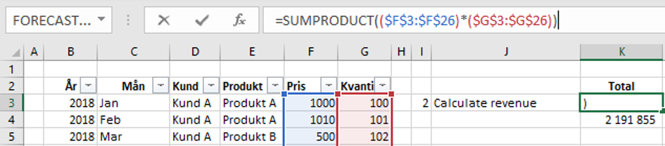
2. Summary with multiplication

In the example below you see that we can also multiply price by number to get the revenue value. I have chosen to have only one exception, i.e. years. What the formula does is that it multiplies line by line plus it selects the sum for the year 2019 only. I use this variant for analytical reports.

If we do not want an exception, the formula becomes the same but without the first parentheses:

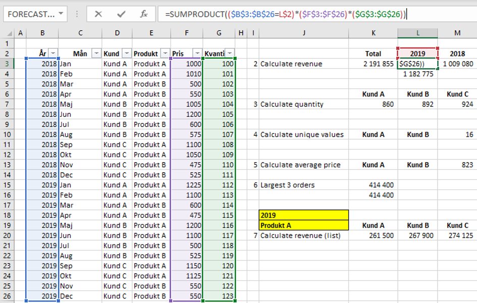
3. Calculate quantity

This variant can be equated with SUMIF, i.e. we sum values with an exception only. I use the method for summaries when we need to have a value quickly.

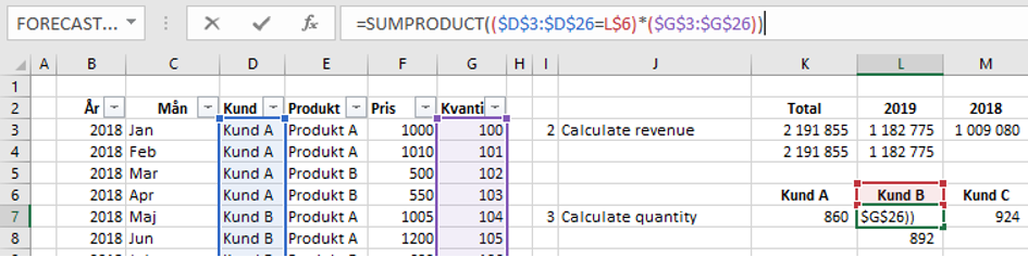
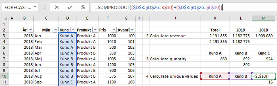
4. Calculate unique values

The example below is a summation variant of NUMBER. The formula looks at how many times customer A and customer B appear in the data. The data area is the customer column and the exception is first customer A and the same logic is then added for customer B. This variant is of a more statistical nature.

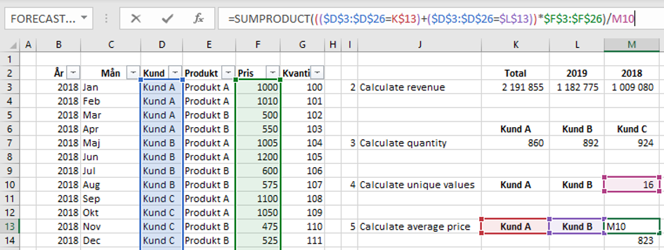
5. Calculate average price

Here we look at a calculation of the average price by first summing up all the price amounts for customer A and B, and then dividing by the number of unique values for the same according to the above example. This variant is also useful for statistical work.

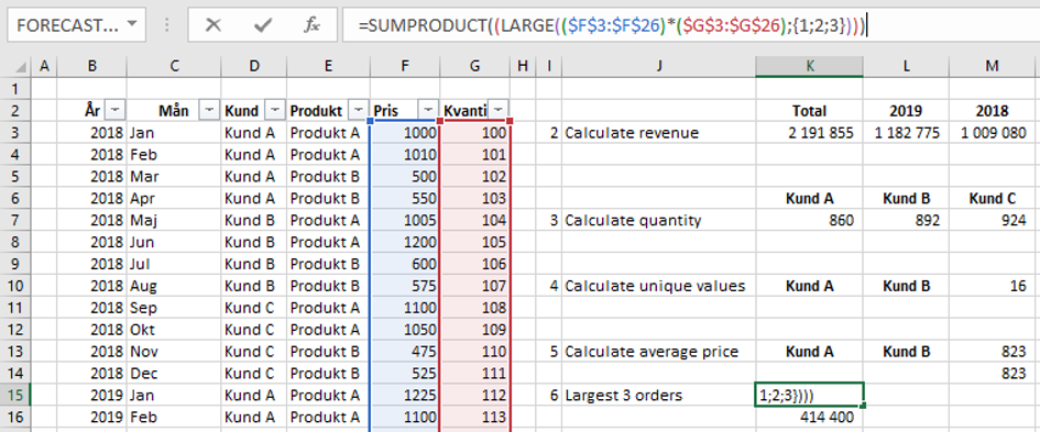
6. Summarise largest orders

In this example we have made a nested formula, and used a formula in the formula. Here we have started with SUMPRODUCT and added the function LARGEST and selected size number 1-3. Observe the number of parentheses that is required and where they are located. This variant is somewhat more complex and can be used to advantage in business analysis.

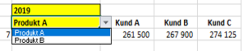
7. Calculate revenue with list function

In this last variant of useful functions with SUMPRODUCT, I have chosen to show how to calculate revenue for different customers and with the choice to adjust year and product in a filter list. We have now made the function dynamic and added in more exceptions and factors that affect the result we get. Working with list functions makes reports much more useful and attractive for presentations directly from Excel.

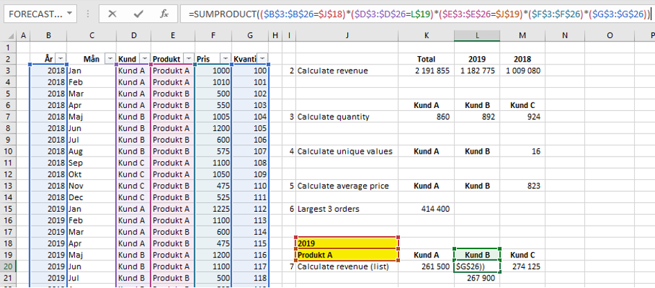
The first 3 parentheses define the exceptions for; year, product, customer and the last two multiply together price and quantity. It takes time to master this type of formula for multiple factors so it is good to try it out and keep track of where the parentheses should be.

In order for you to be able to test the above way of using the formula, I have chosen to attach the file to the above example:

Other tips

The formula has a limit of 255 arrays, which I think is enough for most people. Note that the sum area needs to match vertically and horizontally the array areas you include:

Next post

In this post, I have gone through the benefits of the powerful SUMPRODUCT function and explained what it can actually do and how I use it at work.

Feel free to connect with me on Linkedin and go to Learnesy´s website for more information.

Carl Stiller in collaboration with Learnesy