We have now come to the first posts that deal with reporting. I will show the most common types of reports and how to use formulas to populate the reports in a foolproof way? The new XLOOKUP function is said to be able to replace most functions here, but I still find VLOOKUP to be incredibly useful and most of all easy to apply. XLOOKUP is not available in all versions of Office but a very powerful function.

 

Want to read the post in Swedish? Click here

Look at the lesson in Learnesys course Excel Functions guide, the VLOOKUP function.

https://player.vimeo.com/video/165412503?dnt=1&app_id=122963

^{Use the voucher code cmkstiller for -15% on all Learnesys’ courses}

Performance reporting

As you saw in blog post number 1, a lot of reporting is still done using Excel in some form.
The reporting we do in Excel is still extensive, but done at a basic level as many companies have not landed in Power-BI or Power-Pivot yet.

The reporting that is done today using Excel often has different target groups such as external owners, board, management team, finance department and also the entire company itself if it is results that are to be shared with all employees. This means that there can be many versions of the same result and with different levels of detail. This can be frustrating for a controller group to put together as you spend time on simple reporting instead of analysis. By working with mapping and smart formulas, the time-consuming work can be reduced.

Content of performance reports

Performance reports usually include the following factors or dimensions:

• Accounts and group accounts as well as company specific group accounts
• Scenarios such as actual, forecast, budget
• Currencies such as local currency, USD, Euro
• Organisational level, cost center, division, company, group

If you are going to use one and the same data to be able to set up 4-5 different reports, you can work with mapping the data and then mainly using regular accounts level. See below for examples:

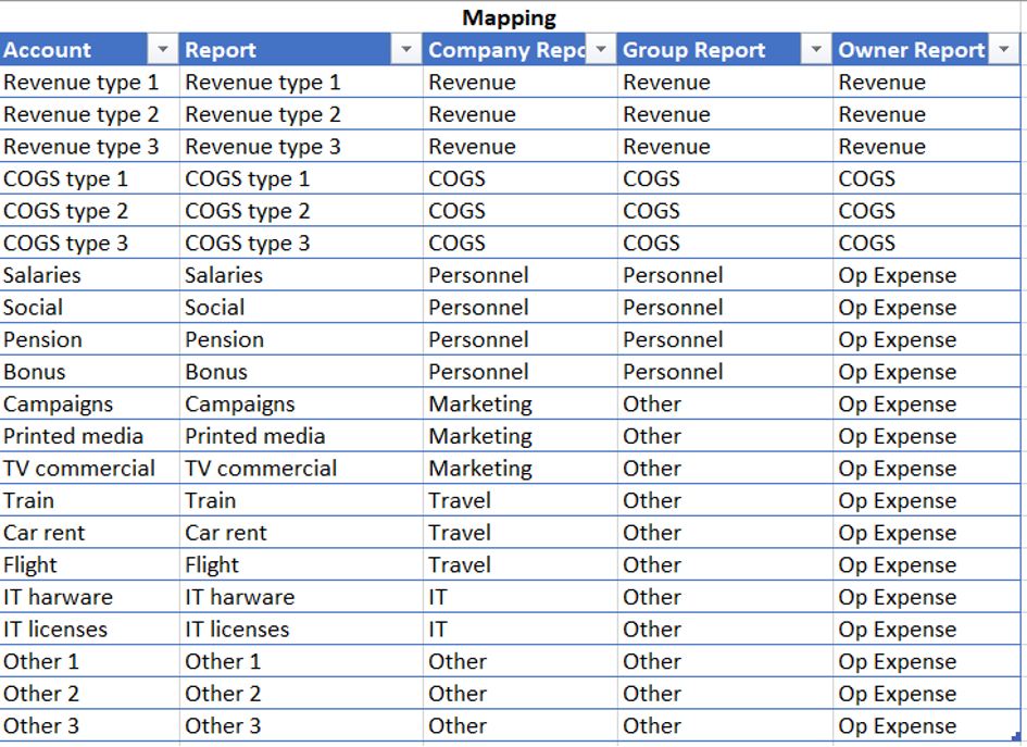
The starting point for the mapping will be at the lowest level, in this case the account level. There are also sub-accounts but I will not deal with those in this post.

Scenarios and currencies

Financial systems provide almost exclusively actual result, so it is always best to verify the actuals in the BI system versus the ERP system and then pull all necessary data only from the BI system. The BI system also often include different currencies, so here you can choose whether you want to pull the data in local or foreign currency depending on the target group.

Suggestions for functions to learn

The different functions that I think you should learn to be able to build good reports and map data are:

• VLOOKUP/HLOOKUP/XLOOKUP
• IF/SUMIF/SUMIFS
• SUMPRODUCT
• PIVOTS

Many people also use INDEX & MATCH and we will gradually go through the various functions in the upcoming posts.

VLOOKUP

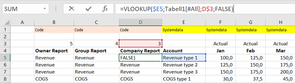
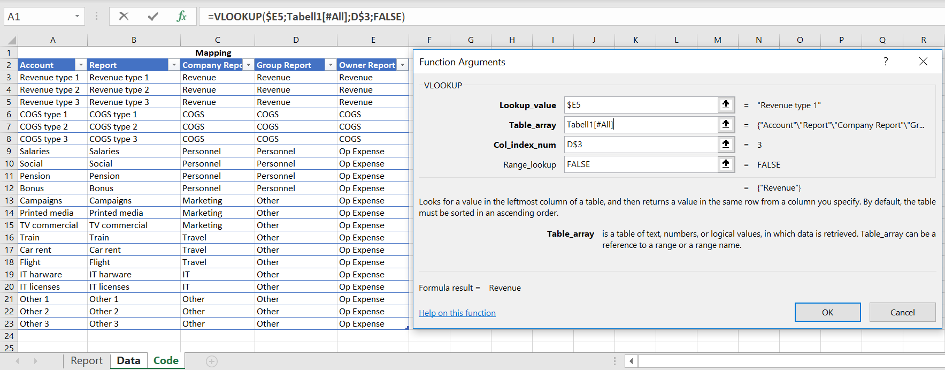
VLOOKUP is one of the formulas I use most frequently since it is extremely efficient to translate or map names or amounts from one table to another. The search value in E5 below looks at the code in the code tab (2^nd picture below) and in its column number “3” to find the group account name “Revenue” to the D-column. If the coding should fail, you often see “#N/A” or “MISSING”. When my mapping contains several columns, I usually work with column numbers and relative cell reference, but you can also type 2 or 3 or whatever number is applicable

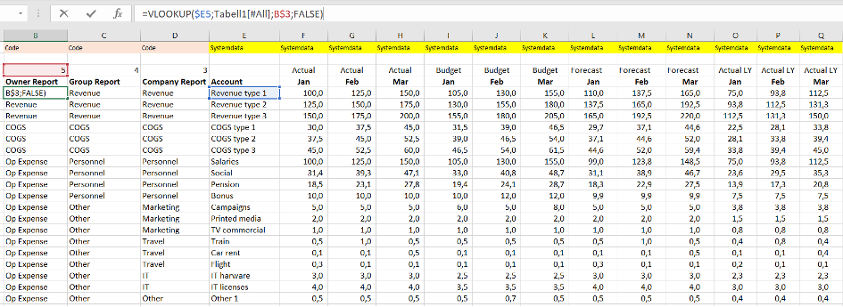
Below you see an example of how I mapped all the report-specific accounts into the raw data.
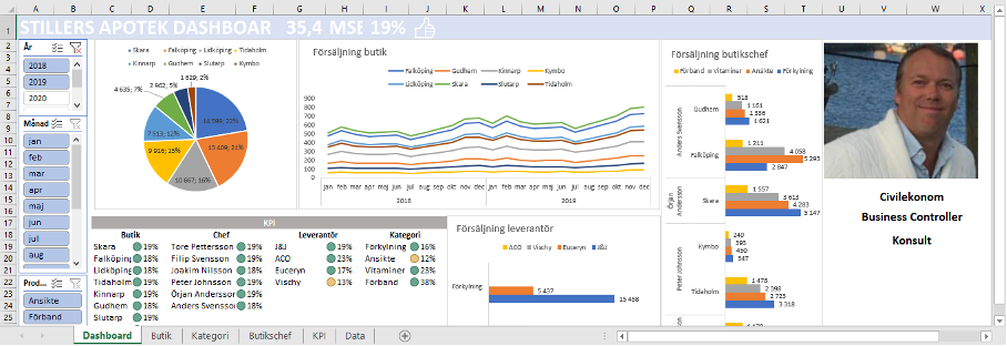
You see that the data consists of months and different scenarios. We can now use this processed information to create dynamic reports for analysis and presentation!

Dynamic reports

Below you see how you can build the reports for the different target groups in one and the samefile with the help of the same data using smart functions.

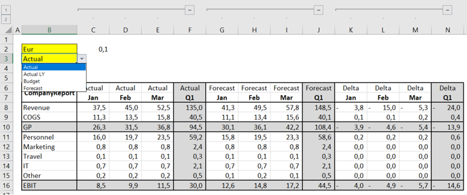
I like to make my reports dynamic, since you can work with the report and that it is not just static information. In this case, I have added filters that you see in yellow. The filters makes it possible to change currency and which scenarios are to be displayed as well as a delta.

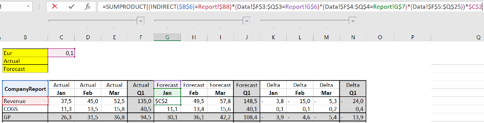
=SUMPRODUCT((INDIRECT($B$6)=Report!$B8)*(Data!$F$3:$Q$3=Report!G$6)*(Data!$F$4:$Q$4=Report!G$7)*(Data!$F$5:$Q$25))*$C$2

I have used my absolute favourite function which is the SUMPRODUCT to populate the report. How the formula works I will explain in a later post. I have also made a nested formula meaning that I have a function in a function. In this case, the INDIRECT function to be able to pick up the different account mappings based on report type.

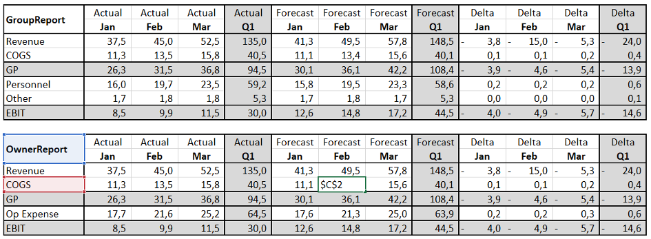
Above you see 2 of 3 reports and that these have a more compressed income statement but that EBIT is still the same.

See below for sample file:

Next post

We have now looked at how to build different target groups’ predefined reports by working smart with mapping and VLOOKUP in Excel. In the next post I will go through the new super function XLOOKUP and explain what it actually can achieve.

Feel free to connect with me on LinkedIn and go to Learnesy´s website for more information.

Carl Stiller in collaboration with Learnesy