Hello, I hope you have a nice working week. This post discusses PivotTables, calculated fields as well includes a tip regarding the equivalent in Power Pivot.

Read the post in Swedish here

Calculated fields

Calculated fields are a function that is perfect to use when you have large amounts of data and where we do not need or want to add columns for calculations in the raw data. We want to make these calculations directly in the PivotTable, which means that the new fields can be rotated just like other factors in the PivotTable. This is especially useful if we have created a table of raw data that is updated every month…then we only need to update our pivot instead of adjusting the raw data. I mainly use calculated fields for:

• Sales analyses
• Margin analysis
• Calculation of delta or changes
• Account reconciliations
• Index calculations

Look at the lesson in Learnesys course The Excel PivotTable guide, Adding a Calculated Field.

 

Example

See below for 5 examples of calculations that are useful in analytical work.

Example 1- margin analysis

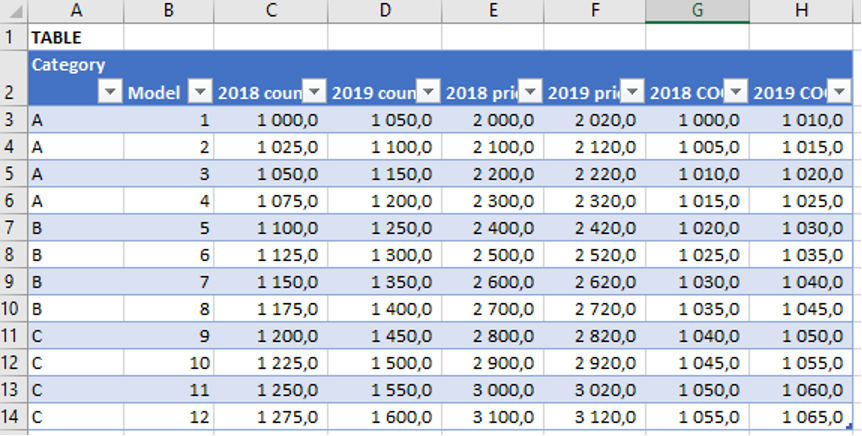
Let’s take an example where we have a data tab with sales information. We can with advantage make this a table before we create our pivot (Ctrl+T). We now want to see the revenue per model for 2018 and 2019, this information however is not in the data, here we only find price and KSV per model and product category.

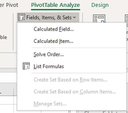
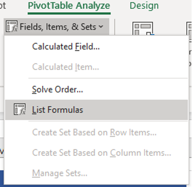
1. We first create an empty pivot with only model and category and then go to the menu tab ” PivotTable Analyze” where we find the below selection…where we select “Calculated fields”.
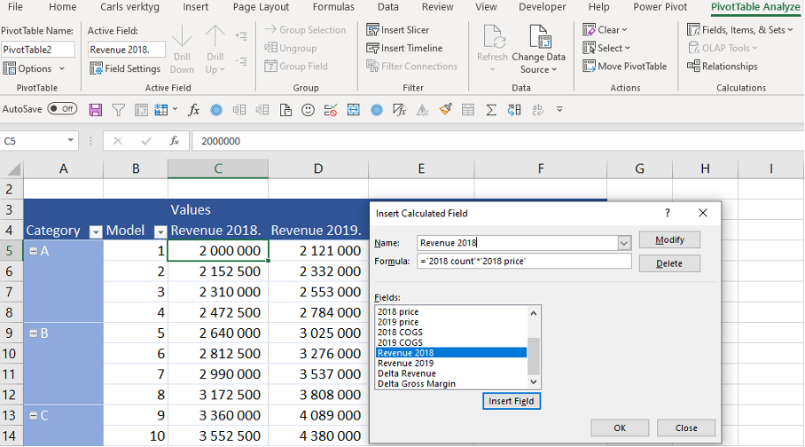
2. We add a name for the field we want to calculate
3. Jump down to the formula field where we multiply price * number and do this for both 2018 and 2019

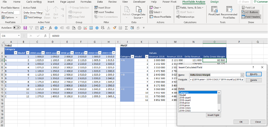
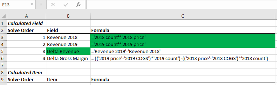
If we instead want to calculate the delta for the gross margin 2018 against 2019, we write the slightly longer formula where we calculate the margin for the two years and then calculate the difference.

= ((‘2019 price’-‘2019 COGS’)*’2019 count’)-((‘2018 price’-‘2018 COGS’)*’2018 count’)

If we were to make this calculation in the data sheet, it would be somewhat more complicated, whereby we now work efficiently with Excel’s functions. Consider if we would have a SQL database linked to the data tab, which I for example had at Apoteksgruppen where I worked with sales statistics. Before I started using calculated fields, the application could freeze several times because it became too much to process.

We can also extract a list of formulas to verify the logic. We see here that in formula 3 we use formula 1 and 2.

Example 2 – percentage increase

We can also calculate the increase or decrease month by month for eg income as below.

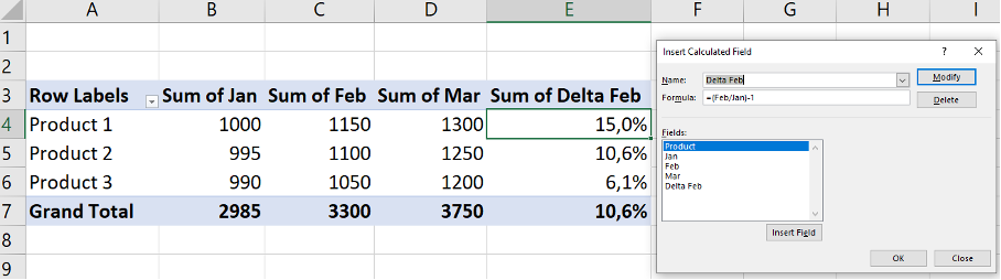
We receive a percentage increase per month here. This type of calculation can also be applied to accumulated data or “Year-on-year”. You can also base it on deviation actual result against budget.

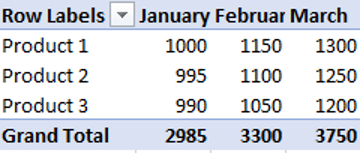
Tip – Name in the table

A useful trick is that if you do not want it to say “Sum of”, you can put in the name and for example write January (note not Jan who already exists).

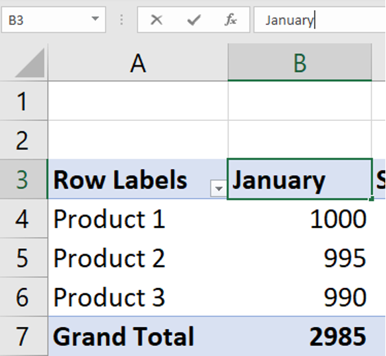
This makes the report look much more pleasant and presentable:

Example 3 – campaign share

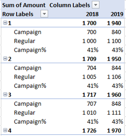
In this case, we have sales data in a table where we have defined whether a model was sold on a campaign or at a regular price. Since we have this data and categorisation of sales type, we need to use the function calculated item.

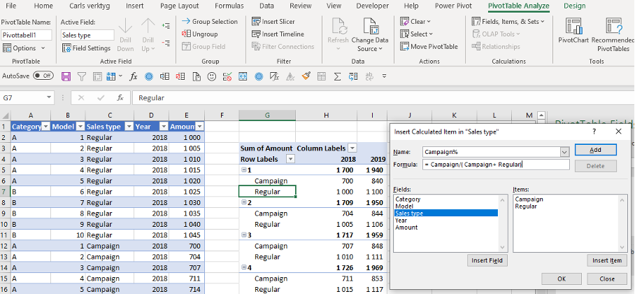
We capture the factors we need for the calculation in the right box that defines the elements of the fields and write our formula according to the image. We get the results below!

Example 4 – Account reconciliation

Normally, at monthly accounts, I usually reconcile accounts, ERP and BI systems, through SUM PRODUCT or VLOOKUP. However, the variant below is good if you have a large amount of data such as 30 cost centers and need to be able to twist and turn the analysis.

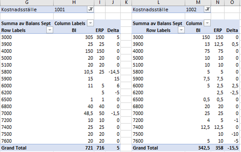
In the following cases, we have only two cost centers and have obtained balances in a tabular form from the ERP system and the BI system. We now want to add a delta between these systems after we’ve set up the PivotTable. NOTE that in order to be able to add a new element to the field for systems, in this example I need to be in cell I4 in the PivotTable, otherwise Excel does not know that this is where a formula should be entered.

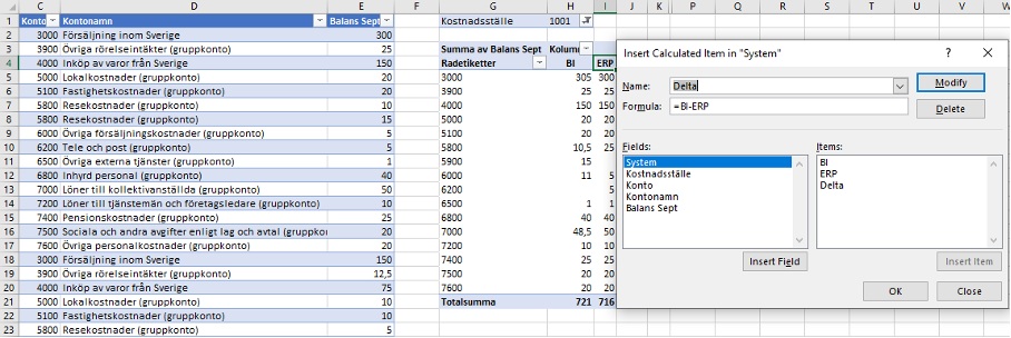
We click OK and the new item is added to the system field and to the PivotTable. We can now filter on cost centers and make our reconciliation. We see that our example has several deviations where the balances are incorrect and where in some cases there are no balances in the BI system.

Time to contact the accounting department and check the export from ERP to the BI system! ?

Example 5 – Calculated fields (dimensions) in PowerPivot

If you have a database with products and product categories, as in example 1 above, then you might want to be able to see the calculations not only per product but also per category. We can not use calculated fields in Excel for this but need to use Power Pivot and DAX formulas. The reason is that the totals will not be correct per category as Excel will sum up all prices per model and multiply by all numbers in one go and thus become too large a total. We will not go through how to use PowerPivot in this post but I think it is worth mentioning how you need to work to get around this issue. It is not uncommon to feel confused for a long time before giving up the calculation in normal Excel.

After uploading the required data and having created relationships in the Excel file, you then need to go to what is called measurements under the Power Pivot tab… you do not work here with analysis for PivotTable. Here you enter = SUMX plus the formula for, for example, the margin calculation.

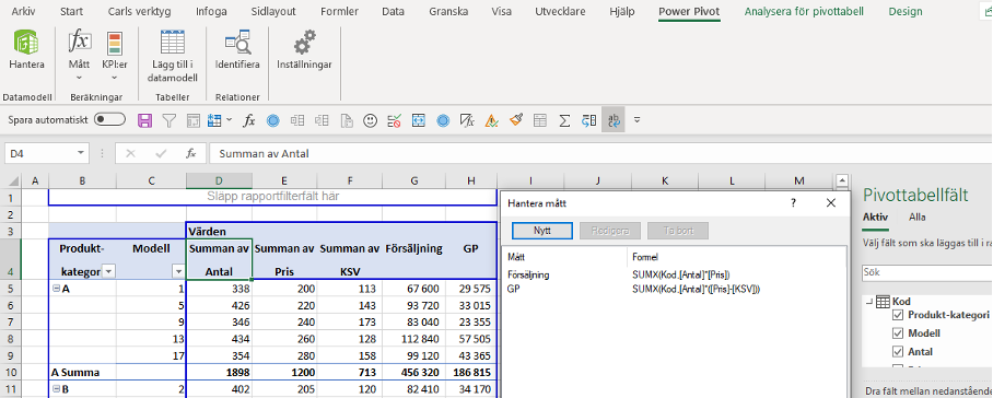
As you can see above, all individual models add up to the correct category total for both sales and GP? .

Next post

Today we have gone through calculated fields and items in PivotTables and how it can streamline your analyses. In the next post I will go through how to use Slices.

Feel free to connect with me on Linkedin and go to Learnesy´s website for more information.

Carl Stiller in collaboration with Learnesy