If you want to try the FV() function yourself or the mathematical formula, and/or recreate the chart above, you can find a file for that below:

<<Material for the article>>

This article covers how to calculate compound interest in Excel in two different ways. There is no generic function for this in Excel; you either have to rely on writing your own formula or use the FV() function. The effect of compound interest is that you earn interest on the interest that, for example, a savings account has already generated. Savings can grow in value both from the interest on the principal and from the interest on previously paid-out interest.

Compound interest is interest calculated on the initial principal of an investment plus all previously earned interest during the period. This is also why people sometimes talk about cumulative interest—interest on interest!

The purely mathematical formula for compound interest looks like this:

where is the initial principal, is the interest rate for a given period (month, year, etc.), and is the number of periods.

Examples of compound interest effects include bank loans, where interest is usually paid several times a year. Since the annual interest rate is divided by the number of periods per year, the effect is that the effective interest rate becomes higher than the advertised annual rate. Another example is investments where dividends are reinvested, resulting in a similar effect. Compound interest is often mentioned together with the snowball effect. Just like a snowball grows bigger every time it rolls through the snow, capital grows with every time period. If you start with a small snowball (small capital), it takes quite a while in the beginning for it to grow, but over time it grows faster and faster. Let’s say you have 10,000 that grows by 10% in the first year. That gives a return of 1,000. If you withdraw that 1,000 right away, the money will continue to grow at the same rate year after year. But if you let the return remain, the next year you will get 1,100. This is what we call exponential growth. The formula above is therefore an exponential function, something that will be visualized later.

To see how the formula works, you can insert values into it. If the initial principal is 10,000, the interest rate is 0.10, and the number of years is 30, we get the following:

A 30-year period gives the following chart:

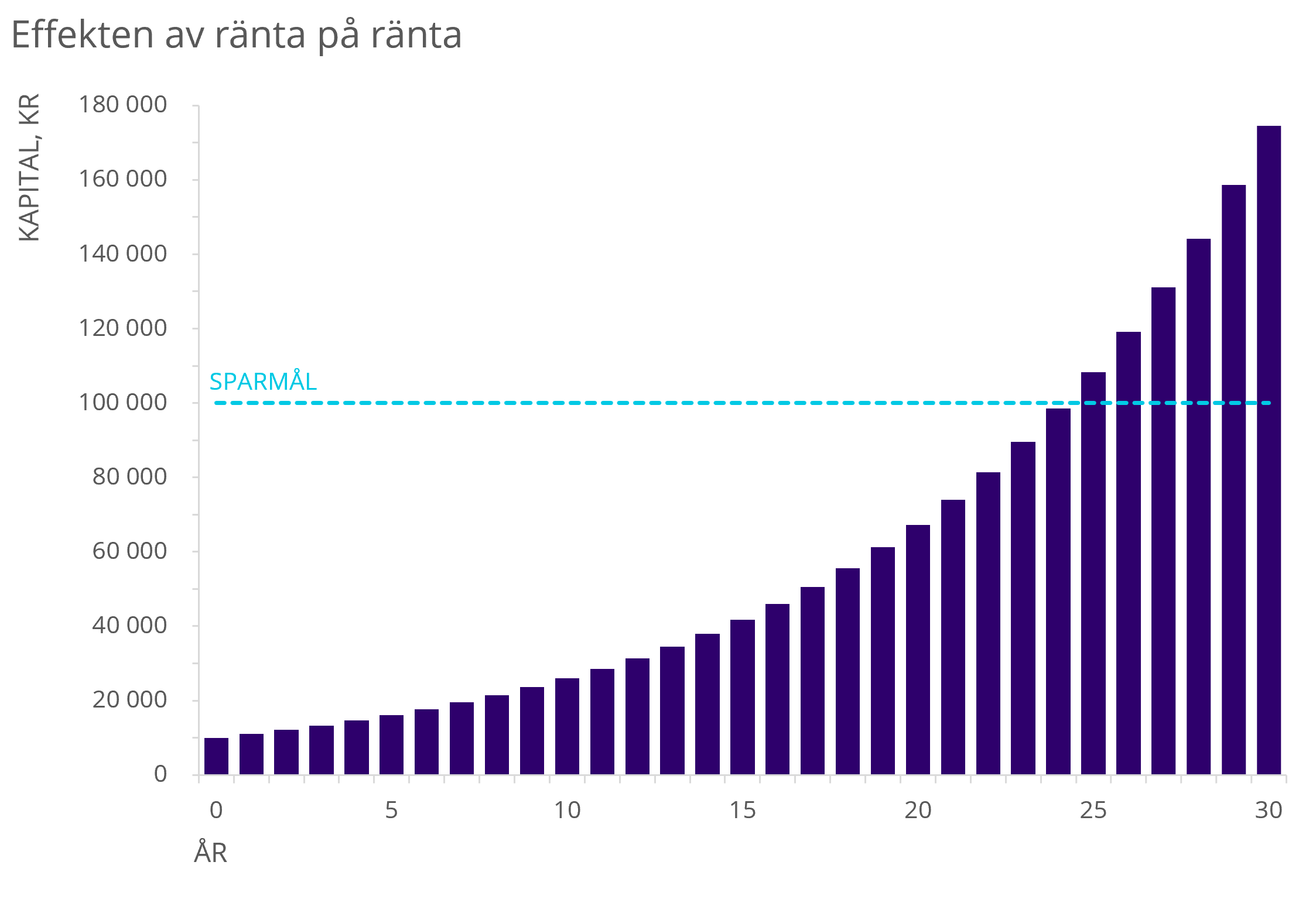
Figure 1: shows the effect of compound interest with a starting capital of 10,000 SEK and a fixed annual interest rate of 10%.

The curve is therefore a good example of the described snowball effect, i.e. the capital increases more drastically with each passing year.

Exponential functions follow the same rules as all other functions. However, exponential functions also have their own unique sub-rules. It is one of the most important functions in mathematics, and differs from perhaps the most important of all: the linear function. In short, it is the independent variable in the exponent that gives the curve its shape.

If you have the graph, you can therefore solve the equation “how many years will it take until I have saved this amount?”. This can also be solved purely mathematically, but that is considered more advanced.

The financial function FV() returns the future value of an investment based on a fixed interest rate. FV() can be used for fixed, recurring payments or for a lump-sum investment.

FV() uses three required arguments and two optional ones. This function and its arguments can be used to calculate compound interest. Here, I will show how you can use four of the five arguments to calculate compound interest spread over 30 years, based on the earlier example:

This corresponds to the “theoretical” value. The function works like this:

Example:                       =FV(0.1, 30, 0, -10000)

As mentioned, there is no generic formula in Excel for calculating compound interest. FV() is usually used to calculate the future value of a loan, i.e. the amount of money you still owe after all repayments have been made. This value is usually (and preferably) 0, since most people do not want to carry debt. The FV() function returns a loan’s future value if we have the other relevant values. Therefore, the function can be used to determine what repayment rate you should maintain in order to be debt-free after x number of years.

It should also be noted that FV() can be trickier to use in examples where the periods are not years but rather quarters or months. In that case, you need to consider how many payments must be made per year. For monthly payments, the syntax looks like this:

=FV(0.1 / 12, years * 12, 0, -10000)

since you must always take into account that there are 12 months in a year.

In Excel Functions Guide, you learn over 90 useful functions. A whole chapter is dedicated to financial functions, including FV(). There is also a lesson specifically on calculating compound interest. In that lesson, compound interest is calculated using a custom-built mathematical formula.

“Since there is no built-in function for it, this lesson will show a way to handle compound interest. We have taken a loan of 150,000 SEK, with an annual interest rate of 7%.

To calculate the annual compound interest, we start by typing equals (=) and selecting the original loan. We then need to multiply the loan by the interest rate, which is 1.07. This gives us the loan plus the 7% annual interest. If we copy the formula down, we can see the compound interest for each year. There is a formula for this, and we use the values below.

We type equals (=), select the loan, multiply by, within parentheses: one plus the interest rate, divided by the periods per year… raised to the power of, within parentheses, the periods per year multiplied by the number of years. As we can see, the value we obtain is the same as in the other method. If we compound monthly, we simply change the periods per year to twelve, and we will see that the result changes even though the number of years remains the same. In this lesson, we have gone through how to handle compound interest in Excel”

In the lesson, another example situation is presented; but to return to the recurring example in this post, I will calculate the investment of 10,000 SEK after 30 years. Feel free to try this formula in the exercise file that belongs to the lesson above. The formula (without any cell references) is:

which results in 174,494 SEK. You can also try replacing the values in the cells instead. In the exercise file, you can also take the opportunity to use FV() in the same way I did in the table. Don’t forget to visualize this with a line chart or a column chart, or combine the two.

I hope this post will help you calculate compound interest. It is relatively straightforward as long as you know the formula and/or use FV(), especially when it is annual compounding. It is also important to understand what compound interest actually is.

If you want to learn more about the courses Learnesy offers, you can do so here.