This article discusses the XLOOKUP function. For a quick lesson on XLOOKUP, you can view the lesson below from Learnesy’s Basic Excel course.

Read the post in Swedish here.

What is XLOOKUP?

The feature was added to Office 365 year 2020 and has since then partially replaced:

• VLOOKUP
• HLOOKUP
• IFERROR
• INDEX&MATCH
• OFFSET

I think you should continue in the way that works well but not be afraid to evaluate new features to see what they can provide and if you can work even more efficiently. I have not let XLOOKUP replace VLOOKUP in my work, however, I use the function when I know it is more efficient. The more I use it, the more uses I find.

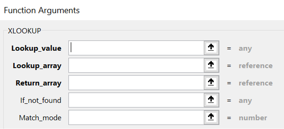
See below for the arguments:

1. Lookup_value (same as VLOOKUP)
2. Lookup_array (same as the first column in VLOOKUP)
3. Return interval (same as after the first column in VLOOKUP)
4. What happens if there is no value to return? (optional)
5. Match mode determines how the values are to be matched (optional)

6. Search mode determines the order in which the search takes place (optional)

Own experience

I have so far used the function when I was working on putting together information that can be found anywhere and when VLOOKUP’s function does not work. For example, when I worked with bonus budgeting last winter, it was useful when I received staff data from HR and salary as well as bonus terms from the CFO.

5 examples

In the explanation below, I will take the bonus calculation for a management team as an example. This is because it is usually the case that you need to capture different factors from different tables that do not always match each other due to the fact that they come from different departments with their special set.

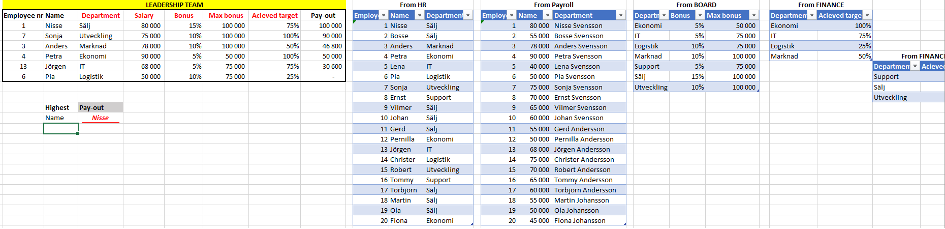
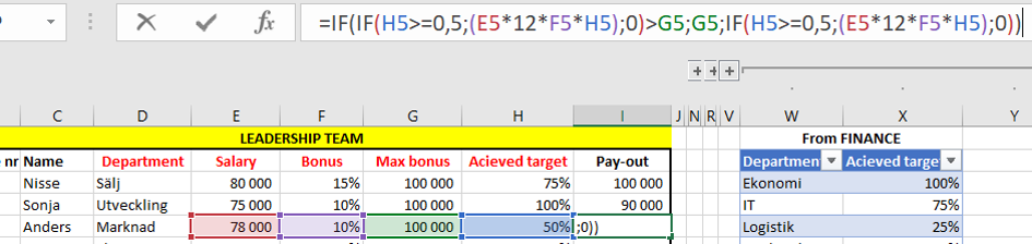
In bonus calculations, you often have the following factors; salary (SEK), bonus share (%), achieved goal (%), maximum bonus (SEK). That is, the bonus is calculated on the salary and the share while taking into account the achieved goal. There is also a ceiling on how high a bonus you can pay out. We have these conditions in our example below, where we first need to populate the missing fields (red text) for the management team and calculate the pay-out. You also want to know who has the highest pay-out.

Example 1: When XLOOKUP replaces VLOOKUP

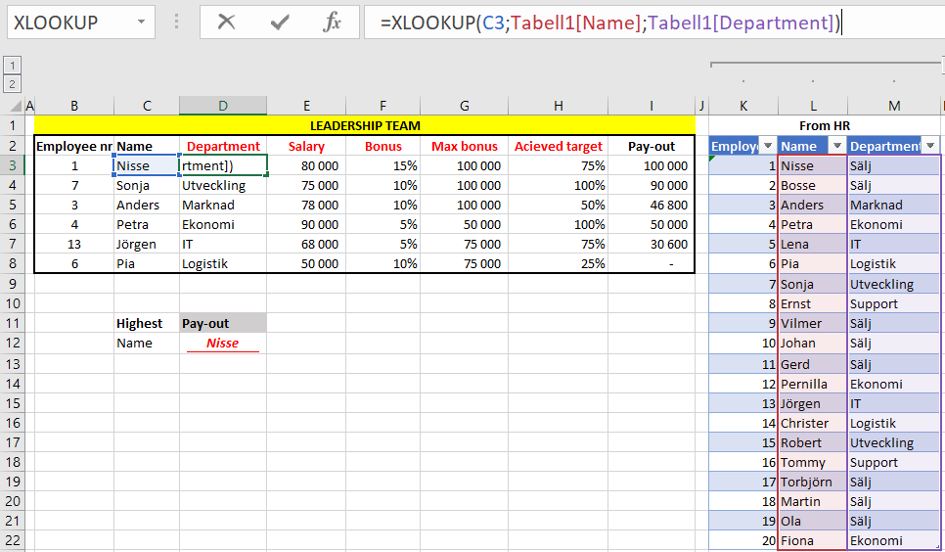
We start with a simple exercise namely, to add the department, which we received from HR. We see below that we only use the three mandatory arguments for this exercise where we only have a single column that returns values. We will soon make it a little more complicated…?.

Example 2: When XLOOKUP replaces VLOOKUP backwards and Wildcard matching

In the example below, you can see that you can capture a value to the left of the LOOKUP value.  This does not work in VLOOKUP (however, I have found a workaround on this). The names of the management group must be found in the table from the Payroll Department and we want to map current salaries.

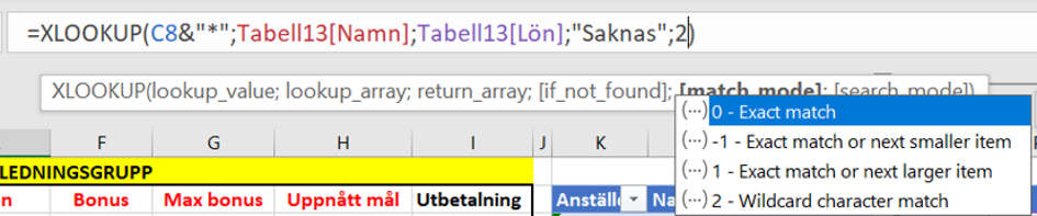
At the same time, our analysis box has only first names and does not completely match payroll info (this situation is very common due to HR systems). We now use Wildcard Matching. This means that we need to select the cell C4 and add & “*”, which means that we start from the existing first name and claim that there may be another name after the first name in the table we are looking in. If we put “*” before C4 then it will be the other way around.

The limitation in this function is if there are several people with the same first name. Note that you can also write; “*” & C3 & “*”, ie Joker on both sides but in our case, we know that we have the first name of everyone in our management team.

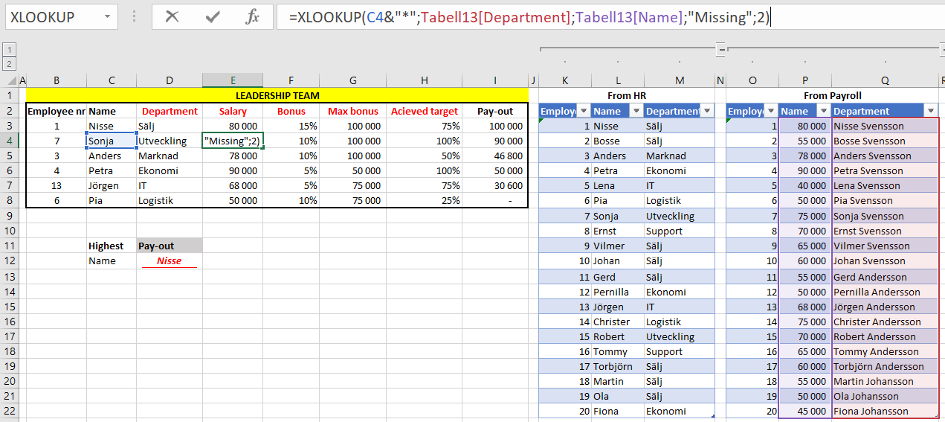
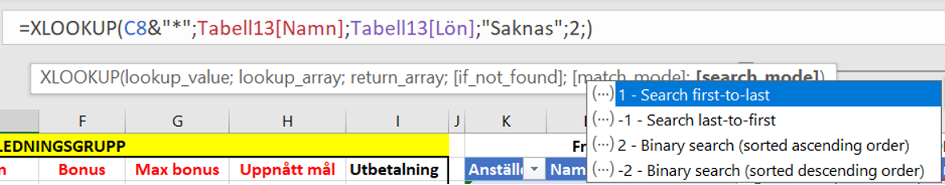
Note that I have chosen to add the optional argument that defines what happens if we do not find a name by writing “Missing”. I have also chosen “2” in the match, which means Joker character matching.

Example 3: When XLOOKUP looks up several factors

The function can, if you select an area with several rows and several columns, find several specified factors as a search value. In the example below, I have marked 2 columns (T and U) as we want to find both the bonus percentage and the maximum bonus per name.

The limitation, as I see it, is that the factors in the compilation need to be the same as in the table and in the same order. That is, F2 needs to be the same as T2 and G2 the same as U2.

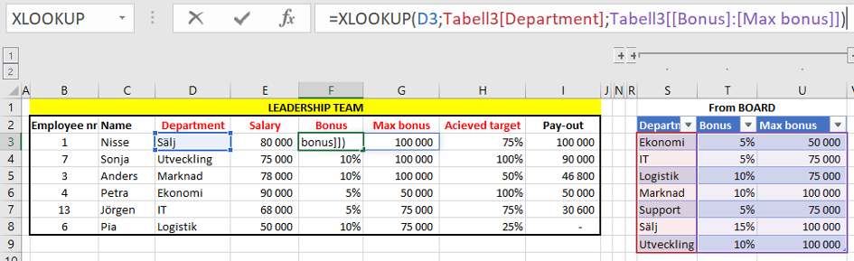
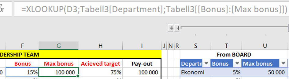
If we enter the formula in F2, it will also be automatically populated in column G and we will see this automation because the formula in G is gray:

The function is great if you have many factors to be found one after the other. However, keep an eye out so it does not go too fast! ?

Example 4: When XLOOKUP uses a nested formula

In this example we see how we can use a nested formula in XLOOKUP. This is because we need to get values from two tables in different places in the Excel file. It is not uncommon to receive the raw data in this way and I have, for the sake of simplicity, placed the small tables next to each other, but they can be in different tabs and also in different files.

=XLOOKUP(D3;Tabell5[Department];Tabell5[Acieved target];XLOOKUP(D3;Tabell6[Department];Tabell6[Acieved target]))

What then does this formula do… yes, we have here used the optional argument If_not_found and written that XLOOKUP (again) should check in a secondary table if it does not find any value… no more complicated than that. I found a video on Youtube where an Excel star from India tested adding 10-15 tables and it worked great.

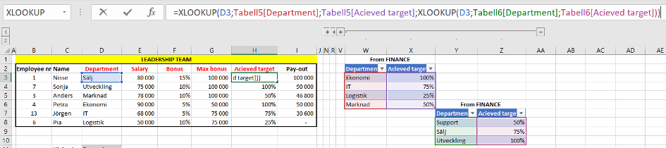
We now see that our calculation for the management team is complete and Nisse is the one who gets the most in bonus as he gets the maximum bonus of SEK 100,000. Nisse has achieved 75% of the target and has a full SEK 80,000 in monthly salary, with which he would have received SEK 108,000 for this if the board had not set a ceiling of SEK 100,000. Pia is the only one in the management team who does not receive a bonus as the requirement is to achieve at least 50% of the goal.

Example 5: When XLOOKUP replaces INDEX & MATCH

Let’s say that we back the band slightly and have not received “Achieved goal” yet and want to simulate who can possibly get the highest bonus. Before the management signs the bonus goals, finance always need to make an impact assessment where they go through what the possible outcome may be and what it means for the employees and in relation to the budget.

We now need to involve the MAX formula in our ?super formula XLOOKUP.

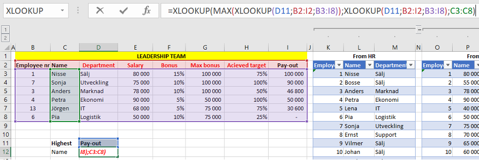
What then happens in this formula? First, we let the formula find out which value is greatest in the pay-out column and then find out who gets that specific pay-out. As you can see, I have marked all the columns as one single area to look in and the finesse of my formula is that I can define via a filter list whether it is payment or salary etc that we want to check.

How does the formula work really…?

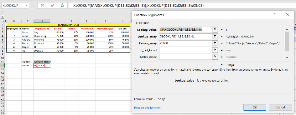
Lookup value

If we look at the function arguments, we start the formula by defining that it is an XLOOKUP function. Then, with the help of XLOOKUP, the MAX formula can find the highest value for the factor that we define in cell D11.

Lookup array

Here XLOOKUP looks for the values, in our case I have set the filter to the achieved target so you see that the values that are visible are 0.75 (75%), 1.0 (100% etc.

Return array

Here, the function finds the names of the people in the selection and who has the highest value.

Conclusion

The focus of this slightly longer post has been XLOOKUP and 5 applications that I most often use it for. Remember that the best way to learn the formula is to temporarily avoid VLOOKUP. Feel free to connect with me on LinkedIn and check out Learnesy’s course catalogue.

Below you can also see the webinar I conducted on behalf of Learnesy. I hope you will learn something new. Please note that this is in Swedish. 

Carl Stiller in collaboration with Learnesy