Today we continue to go through how to “wash data”. The reason why we encounter amounts in non-numeric format is often due to the fact that we have exported data from, for example, an accounting system or saved data in file format such as csv.

Want to read the post in Swedish? Click here

Look at the lesson in Learnesys course Excel Essentials, about SEARCH and REPLACE characters in cells.

---

Determine if the amounts are numeric

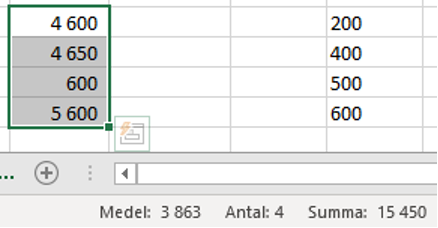
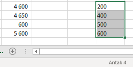
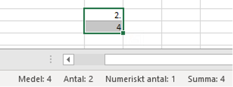
There are several ways to determine if the amounts are in non-numeric format which we looked at in the previous post. The easiest way is to mark the cells with the data and see if they get a sum in the status bar.

• 

• 

By customising the status bar to display the number of numeric numbers, you can also quickly see if the number of cells that are selected is the same as the number of numeric numbers.

Other formats

Formats that I often get when I work for companies with American owners are shown below. As these amounts have different formatting, it is not easy to reformat them, but they need to be processed in another way before they can be reformatted to numeric value.

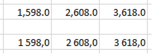
Below you see examples of how certain amounts can look as if they are numerical even though they are of text format and vice versa. It is therefore important to keep your eyes open and do some testing before using the numbers.

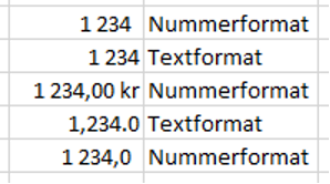
Punctuation instead of comma or comma at thousands

American companies like to place a dollar sign in front of their numbers and to use commas at thousands. Normally you can adjust the custom format quite easily.

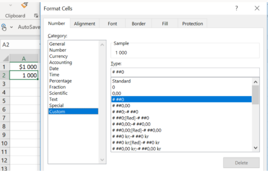
But sometimes it’s a little bit trickier and formatting does not work. They also often use punctuation where we use commas for decimals. This variant can be solved relatively quickly according to the steps below.

Ctrl + F for “Find and replace”… choose comma first and replace with a blank

Then you do the same thing with punctuation but choose comma instead of a blank:

In this process, you need to replace the incorrect comma first, at thousands, adding a comma instead of the punctuation in step two.

Spaces after thousands

In the same way, we can replace blank spaces after a number. We search on space and replace with… nothing. See below:

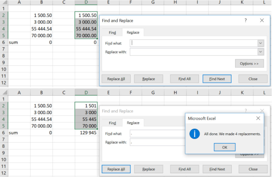
After removing the space, we replace the punctuation with a comma like in the previous example.

Text to column

Text to column is useful when you have different types of information in one and the same cell that you need to separate to be able to use the data for analysis or reporting. See below two examples where we see a space in the first example and that in the second example the number and text are together.

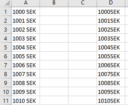
We go to the function “Convert text to column” under the data menu.

Here there are two different choices, either using delimited fields or with a fixed width. In our first case, it works with Delimited fields as we have spaces between the numeric values ​​and the text “SEK”.

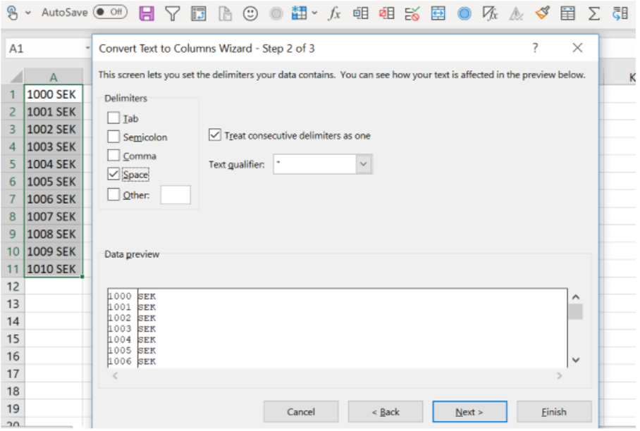
We uncheck the default choice Tab and select Space. You see here that there are several automatic choices but that you can also select “Other” and enter which character should apply.

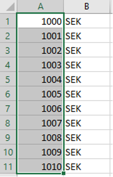
After clicking on finish, we get the end result above.

The second variant is when we see text right next to a numeric value. We can then use the function With fixed width as below

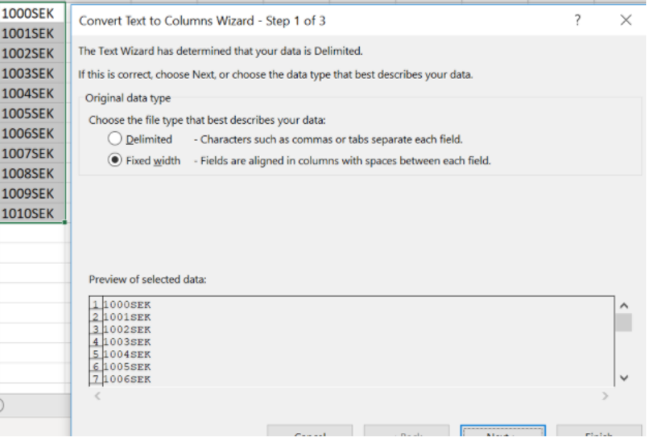
We click four notches on the ruler to get an arrow/line.

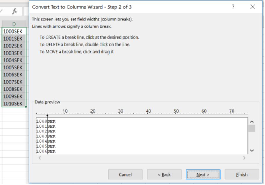
Finally, we click on the next to get a preview or alternatively finish.

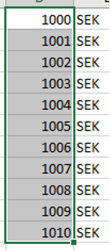
In this variant of the function, we can add several arrows if needed to divide more complicated combinations of numbers, characters and text.

Next post

We have now looked at replacing different formats where punctuation, commas or spaces are making the amounts non-numeric formats. In the next post, we will start looking at reporting and how to easily build visual and informative reports in a simple way in Excel.

Feel free to connect with me on LinkedIn and visit the shop to find an online course that suits you!