📆 14-day money-back guarantee | 🔃 Switch courses anytime | 🔒 Secure payment and fast support

What is the difference between LOOKUP, VLOOKUP, and XLOOKUP?

What is the difference between LOOKUP, VLOOKUP, and XLOOKUP?

What these three functions have in common is that they are all designed to search for values and references. Simply put, XLOOKUP() is an improvement of VLOOKUP(), which in turn is an improvement of LOOKUP(). In this post, I will break down the functions to clarify what differentiates them and when they can be used. To keep it simple, I have chosen to show the functions mostly in their default behavior. The functions will therefore be presented in their purest form, with one or two exceptions.

For those who want to use the same simple dataset, the file is also included with the functions already filled in. However, it is encouraged to test with other datasets as well, preferably larger ones. Although the arguments of these functions are not very difficult to understand, some practice may still be required. The simplicity of primarily LOOKUP() and VLOOKUP() is also what can make working with these functions challenging, which will be examined more closely.

Overview of the functions

LOOKUP() – performs an approximate match in a single row or column and returns the corresponding value from another row/column range.

VLOOKUP() – is a function used to look up data in a vertically organized table. It can be used for approximate, exact, or partial matches. The lookup values must appear in the first column of the table.

XLOOKUP() – is a flexible replacement for LOOKUP(), VLOOKUP(), HLOOKUP(), and the combination of INDEX() / MATCH(). XLOOKUP() can be used for approximate, exact, and partial matches in vertical or horizontal ranges.

How to use LOOKUP

LOOKUP() is used to search in a single row or column and find a value from the same position in another row or column. LOOKUP() has useful default behaviors when solving certain problems. For example, LOOKUP() can be used to retrieve an approximately matched value instead of a position, or to find the last value in a row or column.
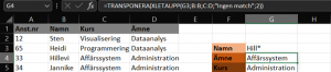
Example 1

In the example below, you can see how to search using an employee’s name to find out which course they are attending.

Note that the video is in Swedish.

=LOOKUP(G3, B:B, C:C)

This function looks up the value in cell G3, compares the value in G3 with the values in column B, and returns the corresponding value from column C on the same row.

The LOOKUP() function accepts three arguments, meaning that all arguments in the example above are used, excluding the optional fourth argument. This can cause the function to behave unexpectedly, which is why I won’t go into further detail here.

It can also be said that LOOKUP() can be used for tables and arrays, though this is not recommended. Additionally, the values should be sorted in ascending order; otherwise, the function may return an incorrect result. Also, make sure that the vectors for the second and third arguments are the same length.

In summary, the function’s weakness is that it is limited to approximate matches. Its strength, however, is that it is multifunctional and flexible. Ironically, this flexibility is something that constrains the otherwise more powerful VLOOKUP() function.

How is VLOOKUP used?

VLOOKUP() is used when you want to find values in a table or array across rows. VLOOKUP() is probably one of the most well-known Excel functions, although it has now been surpassed by the newer XLOOKUP(). Nevertheless, it is still widely used, for better or worse. A positive aspect is that it is easy to use, but like other Excel functions, it can be applied in many different ways. Soon, anyone familiar with the function might want to retrieve multiple values at once or add more criteria. At that point, one will notice its limitations compared to XLOOKUP() or INDEX / MATCH.

VLOOKUP() requires a complete table with lookup values in the first column. This can create difficulties when using the function with multiple criteria. Just like LOOKUP(), VLOOKUP()’s default matching can sometimes return the wrong value. This is why practice is needed—simplicity notwithstanding. To use the function effectively, you need to master the basics.

Example 2

Looking at the example below, you can see that we can get the same result as with LOOKUP(), even though here we are searching for a name and returning an employee number.


=VLOOKUP(G3, A2:D21, 2, FALSE)

The function works like this: what we want to look up; where the function should search; the column number of the value to return; and whether we want an approximate or exact match.

Comparing the tables in the two examples, we see that the employee number and name have switched places. Why is that? Because the VLOOKUP() function cannot retrieve values to the left of a column—it only works to the right. Although VLOOKUP() is an update of LOOKUP(), there are still cases where LOOKUP() may be better suited. VLOOKUP() is more dynamic in handling tables and arrays, and we have the option to choose either an exact or approximate match. We also don’t need to worry about whether the values are sorted, at least not for exact matches. In the VLOOKUP() example, the function performed an exact match, but what if the exact match returns nothing? We could wrap the function in an IF() function and set conditions for what should be returned based on the outcome. XLOOKUP() has a built-in solution for this.

How is XLOOKUP used?

XLOOKUP() is used to find values in a table or row by row. The function searches for a lookup value and returns a result from the same row in another column. Unlike VLOOKUP(), we are not restricted in direction; we can move freely. XLOOKUP() is a flexible and versatile function that can be applied in a wide variety of situations.

We can choose to find an exact, approximate, or partial match. Partial matches use wildcards, such as one or more asterisks. If an exact match is missing, we can get an approximate match, or we can specify that the function should return something else, such as an error message. Like some other Excel functions, XLOOKUP() can return “#N/A” if no value is found. Additionally, unlike many other functions, XLOOKUP() has an optional argument to handle such cases. The user can input a value or string to display instead, e.g., “value not found,” “no result,” etc.

Example 3

Perhaps most useful is that the function can return multiple values, as illustrated in the example below.

=TRANSPOSE(XLOOKUP(G3, B:B, C:D))

We specify the value to search for, the array or range where the value should be searched, and the array or range from which the values should be returned.

Here, the TRANSPOSE() function is also used to get the results as a column vector (vertical) instead of a row vector (horizontal). This is also an example of combining functions, called nesting. XLOOKUP() can thus be nested within other functions. The advantage of XLOOKUP() is that nesting is often less necessary compared to VLOOKUP(). While it is very useful to build long formulas using multiple functions for specific problems, this can quickly become complicated and time-consuming.

There are significant differences between XLOOKUP() and the other two functions. I have already highlighted some differences between LOOKUP() and VLOOKUP(), so now I will focus on the differences between VLOOKUP() and XLOOKUP().

Why is XLOOKUP better to use?

There are big differences between VLOOKUP() and XLOOKUP(), and consequently between XLOOKUP() and LOOKUP(). There are fewer differences between LOOKUP() and VLOOKUP(), so we will set the former aside for now.

Column Index

VLOOKUP() uses the table array as its second argument. This includes the column where we want to find the value. The third argument is the column index, which indicates which column the function should return a value from. VLOOKUP() is programmed to search for the lookup value in the leftmost column of this range and return a value to the right, based on the column index.

XLOOKUP(), on the other hand, separates the lookup array and the return array into two arguments. The lookup array (second argument) contains the values the function searches for, and the return array (third argument) contains the values to return.

Technically, XLOOKUP() does not return values; it returns references, similar to the INDEX() function. This is also one of XLOOKUP()’s strengths.

This separation of lookup and return arrays makes XLOOKUP() more flexible than VLOOKUP(). It doesn’t matter where the columns are located.

Adding Columns

With VLOOKUP(), adding, removing, or moving columns can cause incorrect results. This is not a concern with XLOOKUP() because it doesn’t require a column index.

Error Messages and Default Behaviors

VLOOKUP() has no built-in way to handle missing values; you must wrap it in an IF() or IFERROR() function. XLOOKUP() allows users to specify a return message if the search value is not found.

Also, VLOOKUP() defaults to approximate matching unless otherwise specified, while XLOOKUP() defaults to exact matching. This is one reason VLOOKUP() can more easily produce errors.

Searching from Last Occurrence

XLOOKUP()’s last optional argument can be used to search for the last occurrence of a value, either from bottom-to-top or top-to-bottom. VLOOKUP() cannot do this without additional functions.

Wildcards

XLOOKUP() supports partial matches using wildcards (*).

Note: The image also shows an example of how to use the error message argument (fourth argument). In the fifth argument, you must manually enable wildcard searching.

Weaknesses of XLOOKUP

Its only real weakness is that it is unavailable in older versions of Excel/Office. Therefore, it can still be very useful to first master LOOKUP() and VLOOKUP() and then gradually build more complex formulas. This is especially important if you share spreadsheets with others.

Always be cautious when including headers in your ranges, which applies to XLOOKUP() as well.

Summary Table

Feature VLOOKUP() XLOOKUP()
Exact match by default No Yes
Supports exact match Yes Yes
Requires sorted values Yes, for approximate match Yes, in a very specific case*
Can return incorrect values Yes, with approximate match Yes, in a very specific case*
Returns values to the right of lookup range Yes Yes
Returns multiple values/references No Yes
Searches top-to-bottom Yes Yes
Searches bottom-to-top No Yes
Supports partial match No Yes
Adding columns can break the function Yes No

*For binary searches. If you don’t know what a binary search is, you likely won’t use it.

The table provides an overview of the differences between VLOOKUP() and XLOOKUP(). LOOKUP() should not be forgotten; it’s a simpler version of XLOOKUP(), but lacks many advanced features. There are still cases where LOOKUP() is preferable to VLOOKUP().

XLOOKUP() is clearly an improvement over the other two functions. Compared to LOOKUP(), it allows you to avoid many of the time-consuming formulas that VLOOKUP() requires for more complex problems. While VLOOKUP() and LOOKUP() are still widely used, XLOOKUP() is a necessary upgrade.

I hope this helps you understand the differences between the three functions. Experiment with them, and if you want to learn more, consider taking the Excel Essentials or Excel Functions Guide courses.


Leave a Reply

You must be logged in to post a comment.

More blog posts